Estimating the mean of a bivariate Gaussian

In this tutorial we will use the package ExtensibleMCMC.jl to estimate the mean of a bivariate Gaussian random variable from its 10 observations. We will define a target law and two methods: set_parameters! and loglikelihood that dispatch on our target law. We will then generate some data, show how to parameterize the Markov chain and run the sampler. We will run multiple different samplers, displaying the range of possible algorithms implemented in ExtensibleMCMC.jl. Each time, we will graphically inspect the results.

Defining the target law

Note

In this folder we have already defined some examples of the targets laws and a Gaussian law (with a possibility to estimate its mean and covariance matrix) is one of them. For the pedagogical purposes we define the new BivariateGaussian struct below.

We start from defining the target law.

using Distributions
using ExtensibleMCMC
const eMCMC = ExtensibleMCMC

mutable struct BivariateGaussian{T}
    P::T
    function BivariateGaussian(μ, Σ)
        @assert length(μ) == 2 && size(Σ) == (2,2)
        P = MvNormal(μ, Σ)
        new{typeof(P)}(P)
    end
end

We chose to define it as a mutable struct and use a pre-defined MvNormal struct from Distributions package to encode the probability law. In this way, when parameters change, we may define a new MvNormal struct, with new parameters and then write over the field P of BivariateGaussian, changing it to a new struct with new parameters.

Tip

Depending on the application, you might want to consider changing this convention, define the target law using an immutable struct and have the representation of the probability law be represented by a mutable struct so that its parameters can be changed or, alternatively, have the parameters themselves be represented internally by a mutable vector.

ExtensibleMCMC.jl expects to have two functions implemented for the target law. The first one is a setter of new parameters

function eMCMC.set_parameters!(gsn::BivariateGaussian, loc2glob_idx, θ)
    μ, Σ = params(gsn.P)
    μ[loc2glob_idx] .= θ
    gsn.P = MvNormal(μ, Σ)
end

Here, loc2glob_idx is a vector of indices pointing to parameters that are to be updated. For instance, if the MCMC step concerns only entries 3 and 6 of the 10 dimensional parameter vector θ, then loc2glob_idx=[3,6]. The second expected method is evaluation of the log-likelihood that extends the method defined in Distributions for the target law:

function Distributions.loglikelihood(gsn::BivariateGaussian, observs)
    ll = 0.0
    for obs in observs
        ll += logpdf(gsn.P, obs)
    end
    ll
end

Here, logpdf is defined in Distributions and works by the virtue of typeof(gsn.P) <: MvNormal.

That's it! We're good to go!

Generating the data

We may simulate some test data. The important point is that unless you overload the update functions yourself, the data should be stored in the format of a NamedTuple with fields P containing the target law and obs with a vector of observations.

using Random
Random.seed!(10)
μ, Σ = [1.0, 2.0], [1.0 0.5; 0.5 1.0]
trgt = MvNormal(μ, Σ)
num_obs = 10

data = (
    P = BivariateGaussian(rand(2), Σ),
    obs = [rand(trgt) for _ in 1:num_obs],
)

In here we set the mean of P to random vales. The actual values don't matter and will be overwritten by the θinit—the initial guess for the mean.

Parametrizing the MCMC sampler

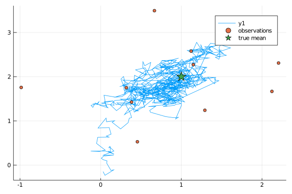
We will start with a simple Metropolis-within-Gibbs algorithm that does single-site updates (alternately updating the two coordinates of the mean) and we will run it for $10^3$ iterations. We will also use improper flat priors.

This can be simply encoded as follows:

mcmc_params = (
    mcmc = MCMC(
        [
            RandomWalkUpdate(UniformRandomWalk([1.0]), [1]; prior=ImproperPrior()),
            RandomWalkUpdate(UniformRandomWalk([1.0]), [2]; prior=ImproperPrior()),
        ]
    ),
    num_mcmc_steps = Integer(1e3),
    data = data,
    θinit = [0.0, 0.0],
)

Note

(a single update of coordinate 1) + (a single update of coordinate 2) == a single MCMC iteration

Running the sampler

With parameterization of the sampler in place, running it is a one-liner

workspace, local_workspaces = run!(mcmc_params...)

Inspecting the results

The output of the sampler is a global Workspace and all local Workspaces. The global workspace holds the entire history of the chain. We can plot it, together with the observations and the true mean to see if we've done OK.

using Plots
function plot_results(ws)
    θhist = collect(Iterators.flatten(ws.sub_ws.state_history))
    p = plot(map(x->x[1], θhist), map(x->x[2], θhist))
    scatter!(map(x->x[1], data.obs), map(x->x[2], data.obs), label="observations")
    scatter!(map(x->[x], μ)..., label="true mean", marker=:star, ms=10)
    display(p)
end
plot_results(workspace)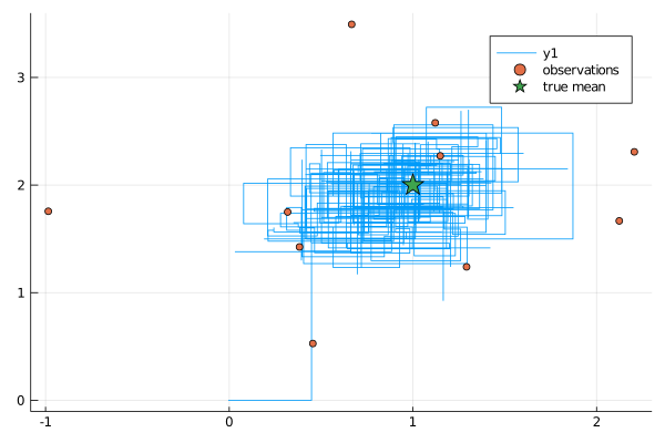

simple_unif_rw

It turns out we did!

Mis-specification of hyper-parameters and adaptation

One of the reasons why we did relatively well in recovering the posterior over the mean parameter was because our proposals were quite decent. However, finding good proposals is a delicate issue. For the uniform random walker this translates to finding a good value for the half-range of steps ϵ. What happens if we set it to too small?

mcmc_params = (
    mcmc = MCMC(
        [
            RandomWalkUpdate(UniformRandomWalk([0.1]), [1]; prior=ImproperPrior()),
            RandomWalkUpdate(UniformRandomWalk([0.1]), [2]; prior=ImproperPrior()),
        ]
    ),
    num_mcmc_steps = Integer(1e3),
    data = data,
    θinit = [0.0, 0.0],
)

workspace, local_wss = run!(mcmc_params...)
plot_results(workspace)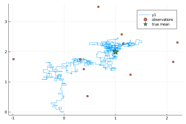

simple_unif_rw_too_small_epsilon

Well, we can see that we are much much slower in exploring the posterior. Finding ϵ by hand might be problematic and to this end there are standard adaptation techniques that target fixed acceptance rate of the sampler by adjusting the ϵ parameter. We can turn such adaptive schemes on using ExtensibleMCMC and then no matter that we start from a mis-specified ϵ, after some burn-in we should find much better candidates for it.

mcmc_params = (
    mcmc = MCMC(
        [
            RandomWalkUpdate(
                UniformRandomWalk([0.1]), [1];
                prior=ImproperPrior(),
                adpt=AdaptationUnifRW(
                    [0.0];
                    adapt_every_k_steps=50,
                    scale=0.1,
                ),
            ),
            RandomWalkUpdate(
                UniformRandomWalk([0.1]), [2];
                prior=ImproperPrior(),
                adpt=AdaptationUnifRW(
                    [0.0];
                    adapt_every_k_steps=50,
                    scale=0.1,
                ),
            ),
        ]
    ),
    num_mcmc_steps = Integer(1e3),
    data = data,
    θinit = [0.0, 0.0],
)

workspace, local_wss = run!(mcmc_params...)
plot_results(workspace)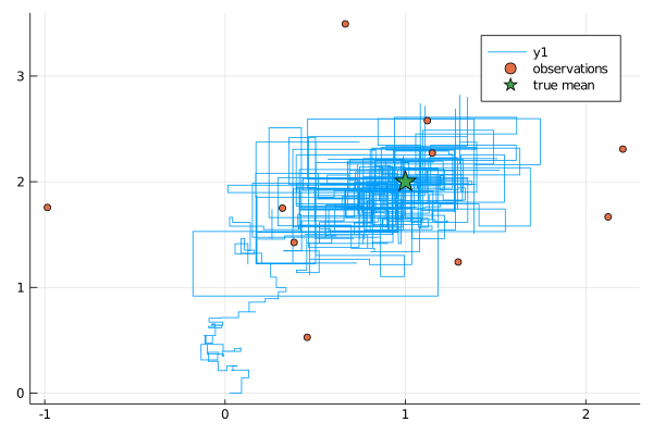

simple_unif_rw_adpt

Gaussian random walk proposals with single-site updates

Sampling from the uniforms may be easily substituted with sampling from Gaussians as the following example demonstrates

mcmc_params = (
    mcmc = MCMC(
        [
            RandomWalkUpdate(
                GaussianRandomWalk([1.0]), [1];
                prior=ImproperPrior(),
            ),
            RandomWalkUpdate(
                GaussianRandomWalk([1.0]), [2];
                prior=ImproperPrior(),
            ),
        ]
    ),
    num_mcmc_steps = Integer(1e3),
    data = data,
    θinit = [0.0, 0.0],
)

workspace, local_wss = run!(mcmc_params...)
plot_results(workspace)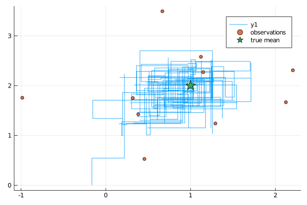

simple_gsn_rw

Bivariate random walk proposals

Naturally, it might be desirable to substitute single-site updates with joint updates. This is again very easily implementable:

using LinearAlgebra
mcmc_params = (
    mcmc = MCMC(
        [
            RandomWalkUpdate(
                GaussianRandomWalk(0.5*Diagonal{Float64}(I, 2)), [1,2];
                prior=ImproperPrior(),
            ),
        ]
    ),
    num_mcmc_steps = Integer(1e3),
    data = data,
    θinit = [0.0, 0.0],
)

workspace, local_wss = run!(mcmc_params...)
plot_results(workspace)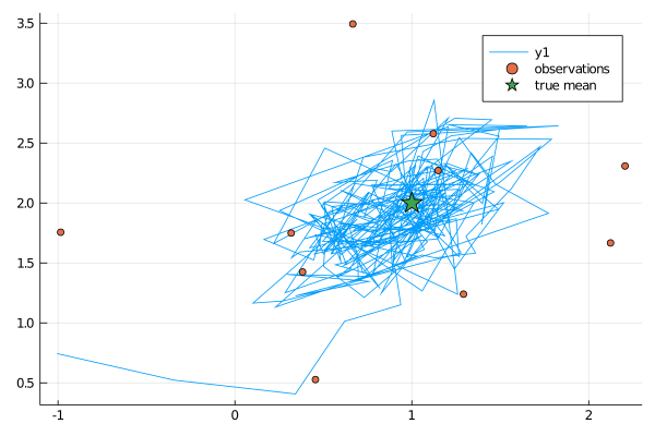

biv_gsn_rw

Of course, the higher the dimension of the proposals the more difficult it becomes to find a suitable covariance matrix for them. For instance, this is what happens if the covariance is not scaled suitably:

using LinearAlgebra
mcmc_params = (
    mcmc = MCMC(
        [
            RandomWalkUpdate(
                GaussianRandomWalk(0.001*Diagonal{Float64}(I, 2)), [1,2];
                prior=ImproperPrior(),
            ),
        ]
    ),
    num_mcmc_steps = Integer(1e3),
    data = data,
    θinit = [0.0, 0.0],
)

workspace, local_wss = run!(mcmc_params...)
plot_results(workspace)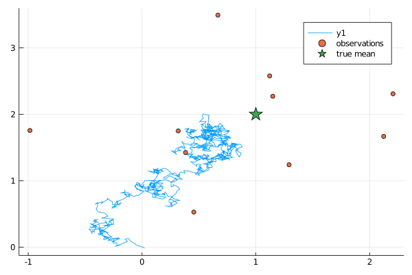

biv_gsn_rw_too_small

Haario-type adaptation for multivariate Gaussian random walk proposals

We may however employ Haario-type adaptive schemes very easily to learn the covariance in an adaptive way.

mcmc_params = (
    mcmc = MCMC(
        [
            RandomWalkUpdate(
                GaussianRandomWalkMix(
                    0.01*Diagonal{Float64}(I, 2),
                    0.01*Diagonal{Float64}(I, 2)
                ),
                [1,2];
                prior=ImproperPrior(),
                adpt=HaarioTypeAdaptation(
                    rand(2);
                    adapt_every_k_steps=50,
                    f=((x,y,z)->(0.01+1/y^(1/3))),
                ),
            ),
        ]
    ),
    num_mcmc_steps = Integer(1e3),
    data = data,
    θinit = [0.0, 0.0],
)

workspace, local_wss = run!(mcmc_params...)
plot_results(workspace)

biv_gsn_rw_adpt