Sampling diffusion trajectories

This package extends functions Random.rand! and Base.rand to sampling of trajectories of diffusion processes.

Trajectories

The containers for sampled trajectories are instances of Trajectory from the package Trajectories.jl. The functions exported by Trajectories.jl are re-exported by this package. The most literal way of defining trajectories is to directly pass already initialized and sized containers (or iterators), for instance

tt = 0.0:0.01:1.0
xx = [zeros(Float64, 10) for _ in tt]
path = trajectory(tt, xx)

However, we may also be more concise and let trajectory initialize the path containers for us:

# for mutable types we need to pass DataType as well as dimension
path_mutable = trajectory(tt, Vector{Float64}, 10)
# for immutable types the dimension is inferred from the DataType
path_mutable = trajectory(tt, SVector{10,Float64})

Finally, if we are initializing containers for a specific diffusion, then we may utilize the default types defined for this law together with information about diffusion's dimensions. For instance:

P = Lorenz(10.0, 28.0, 8.0/3.0, 1.0)
paths = trajectory(tt, P)
XX, WW = paths.process, paths.wiener

Or optionally specify the types ourselves:

P = Lorenz(10.0, 28.0, 8.0/3.0, 1.0)
paths = trajectory(
    tt,
    P,
    Vector{Float64}, # process DataType
    Vector{Float64}, # Wiener DataType
)
X, W = paths.process, paths.wiener

Note

You can also define multiple trajectories at once by passing multiple time segments, for instance

dt = 0.01
paths = trajectory([0.0:dt:1.0, 1.0:dt:2.0, 2.0:dt:3.0], P)
# XX below contains three trajectories and so does WW
XX, WW = paths.process, paths.wiener

Tip

If you need to call diffusion samplers multiple times (because you are using them, say, in an MCMC setting), then initializing trajectories once and passing them around to sampling functions will massively improve the overall performance of your algorithms. However, if all you want to do is sample the trajectory once or a couple of times, then you don't need to worry about initializing trajectories yourself and let it be done by the rand function.

The time vector and path vector can be inspected by accessing fields t and x respectively:

_time, _path = XX.t, XX.x

See the README.md of Trajectories for more details regarding other functionality implemented for Trajectory'ies.

Sampling Wiener process

In this package sampling of diffusion paths is always done on the basis of sampling the Wiener process first, treating it as a driving Brownian motion and then solve!ing the trajectory of the process based on that. The simplest way of sampling a Wiener process is to call:

y1 = ... # define a starting point
W = rand(Wiener(), tt, y1)

The dimensions and DataType of the Wiener process's trajectory are going to be inferred from the starting point y1.

Most often however, we need to sample the standard Brownian motion. For that reason we may omit y1 and it will be initialized to zero. In this case rand will use information contained in the struct Wiener to infer the dimension and DataType, for instance:

W = rand(Wiener(4, ComplexF64), tt)

to sample a four-dimensional complex-valued Brownian motion (with Float64 complex numbers).

Warning

If y1 is not specified the DataType of state space will be set to SVector by default. To change this default behaviour you must overwrite the zero function to:

Base.zero(w::Wiener{D,T}) where {D,T} = zeros(T, D)

say, to use Vectors instead.

Alternatively, to avoid implicit allocation of space by rand we may pass a pre-initialized Trajectory to rand!:

rand!(Wiener(), W)
# OR
rand!(wiener(), W, y1) # The first letter in `Wiener()` may be capital or not

Note that in this case there is no need to decorate Wiener with additional type and dimension information as it is automatically inferred from the Trajectory container.

Sampling diffusion processes

The simplest way of sampling a diffusion trajectory is to call:

P = Lorenz(10.0, 28.0, 8.0/3.0, 1.0)
y1 = ... # define a starting point
tt = 0.0:0.001:10.0
X = rand(P, tt, y1)

The type used for states is going to be inferred from the starting point and the dimensions of the Wiener and diffusion processes will be inferred from P. The decision about in-place vs out-of-place computation will be made based on the inferred type.

Note

y1 can also be left unspecified, then, the trajectory will start from zero and the default diffusion type of P will be used. Nonetheless, for many diffusion laws starting from zero might not make much sense, so this use is discouraged.

rand for diffusions is a convenience function that wraps:

initialization of trajectories X and W for the diffusion and Wiener paths respectively
sampling Wiener path W
solve!ing the path X from the driving Brownian motion based on the Euler-Maruyama scheme.

If you care about performance issues—say X needs to be re-sampled multiple times—then you might want to perform these steps by hand. I.e.

# initialize containers:
X, W = trajectory(tt, P)
y1 = @SVector [-10.0, -10.0, 25.0]
# sample Wiener path:
rand!(Wiener(), W)
# solve for the process trajectory
DD.solve!(X, W, P, y1) # additionally pass `buffer` for in-place computations

Calling rand! and DD.solve! over and over again is much quicker than calling rand multiple times.

Tip

rand and rand! functions by default use the default pseudo-random number generator from the package Random.jl. If you wish to use your own pseudo-random number generator then pass it as an additional first argument, for instance: rand(RNG, Wiener(), tt).

Plotting the results

We provide plotting recipes for the Trajectory objects, so the plot function can be used to visualize the sampled trajectories very easily. Pass Val(:vs_time) to plot multiple (or single) trajectories vs time variable. Pass Val(:x_vs_y) to plot two coordinates against each other. Specify coordinates with a named argument coords. Otherwise, decorate your plots as you would otherwise by calling a plot function. For instance, to plot X[1] against X[3] call:

using Plots
plot(X, Val(:x_vs_y); coords=[1,3])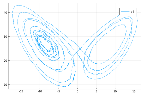

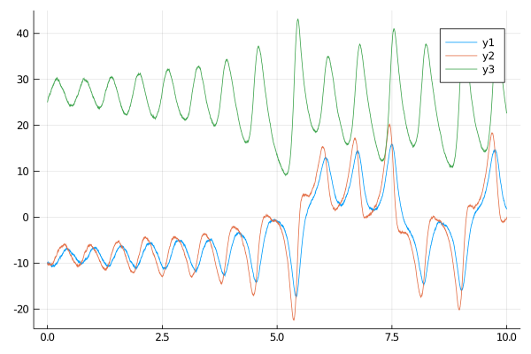
lorenz_x_vs_y

To plot all coordinates against time call:

plot(X, Val(:vs_time))

lorenz_vs_time