Prokaryotic autoregulatory gene network
Chemical Langevin equation for a simple system describing production of a protein that is repressing its own production. The process under consideration is a $4$-dimensional diffusion driven by an $8$-dimensional Wiener process. The stochastic differential equation takes a form:
where $\circ:\RR^d\to \RR^d$ is a component-wise multiplication:
the custom operation $\odot:\RR^{d\times d'}\to\RR^{d\times d'}$ is defined via:
the function $\gamma:\RR^d\to \RR^d$ is a component-wise square root:
$S$ is the stoichiometry matrix:
and the function $h$ is given by:
The chemical Langevin equation above has been derived as an approximation to a chemical reaction network
with reactant constants given by the vector $\theta$.
Can be imported with
@load_diffusion ProkaryoteExample
using DiffusionDefinition
using StaticArrays, Plots

@load_diffusion Prokaryote
θ, K = [0.1, 0.7, 0.35, 0.2, 0.1, 0.9, 0.3, 0.1], 10.0
P = Prokaryote(θ..., K)
tt, y1 = 0.0:0.001:10.0, @SVector [8.0, 8.0, 8.0, 5.0]
X = rand(P, tt, y1)
plot(X, Val(:vs_time), label=["RNA" "P" "P₂" "DNA"], size=(800,300))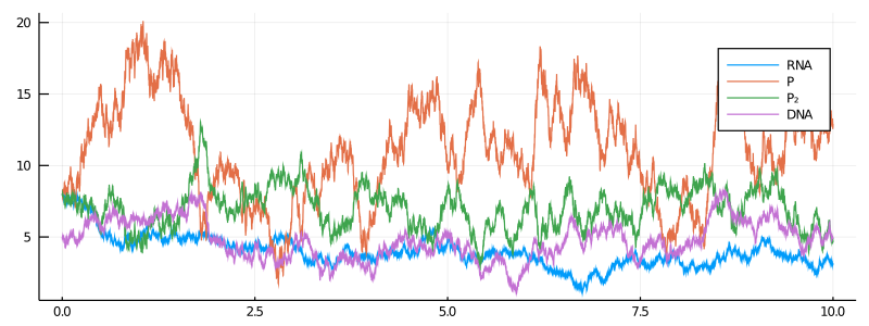
Auxiliary diffusion
We additionally define a linear diffusion that can be used in the setting of guided proposals. It is defined as a solution to the following SDE:
...