Installation

] add DiffusionDefinition

Defining the process

To define a diffusion law use a macro @diffusion_process:

using DiffusionDefinition
const DD = DiffusionDefinition

@diffusion_process OrnsteinUhlenbeck begin
    # :dimensions is optional, defaults both process and wiener to 1 anyway
    :dimensions
    process --> 1
    wiener --> 1

    :parameters
    (θ, μ, σ) --> Float64
end

This will define a struct OrnsteinUhlenbeck and announce to Julia that it represents a one-dimensional diffusion process driven by a one-dimensional Brownian motion and that it depends on 3 parameters of type Float64 each.

To complete characterization of a diffusion law we define the drift and diffusion coefficients:

DD.b(t, x, P::OrnsteinUhlenbeck) = P.θ*(P.μ - x)
DD.σ(t, x, P::OrnsteinUhlenbeck) = P.σ

We will also specify a default datatype for convenient definition of trajectories

DD.default_type(::OrnsteinUhlenbeck) = Float64
DD.default_wiener_type(::OrnsteinUhlenbeck) = Float64

Sampling trajectories under the diffusion law

Use the function rand to sample the process

tt, x0 = 0.0:0.01:100.0, 0.0
P = OrnsteinUhlenbeck(2.0, 0.0, 0.1)
X = rand(P, tt, x0)

Plotting the trajectories

Plotting may be done with any supported backend via function plot. Plotting recipes are provided which make sure that the output of rand (of the datatype trajectory) is understood by plot. For instance, to plot all diffusion coordinates (in case above only one) against the time variable write

using Plots
gr()
plot(X, Val(:vs_time))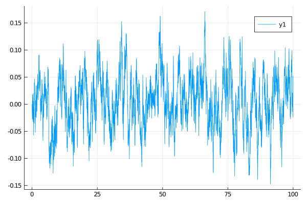

Repeated sampling

The package is implemented with the setting of Markov chain Monte Carlo methods in mind. Consequently, methods are built to be as efficient as possible under the setting of repeated sampling of trajectories. To fully leverage this speed you need to pre-allocate the containers for trajectories:

X, W = trajectory(tt, P)

and then sample the process by:

1. drawing the driving Brownian motion W,
2. and then, solve!ing the path X from the Wiener path W

Wnr = Wiener()
rand!(Wnr, W)
DD.solve!(X, W, P, x0)

Sampling trajectories multiple times becomes very efficient then, for instance:

julia> function foo(Wnr, W, X, P, x0)
           for _ in 1:10^4
               rand!(Wnr, W)
               DD.solve!(X, W, P, x0)
           end
       end
foo (generic function with 1 method)
julia> using BenchmarkTools
julia> foo($Wnr, $W, $X, $P, $x0)
  1.840 s (0 allocations: 0 bytes)

i.e. $2$ seconds to sample $10\, 000$ trajectories, each revealed on a time-grid with $10\, 001$ points (tested on an Intel(R) Core(TM) i7-4600U CPU @ 2.10GHz).