Lotka-Volterra
A simple, scalar-valued predator-prey model.
Can be called with
@load_diffusion LotkaVolterraExample
using DiffusionDefinition
using StaticArrays, Plots

@load_diffusion LotkaVolterra
θ = [2.0/3.0, 4.0/3.0, 1.0, 1.0, 0.1, 0.1]
P = LotkaVolterra(θ...)
tt, y1 = 0.0:0.001:30.0, @SVector [2.0, 0.25]
X = rand(P, tt, y1)
plot(X, Val(:x_vs_y))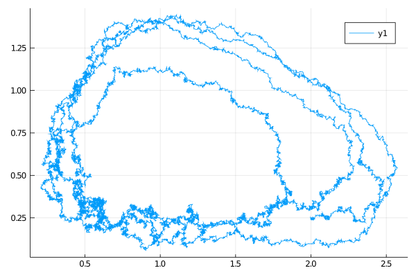
Auxiliary diffusion
We also provide a linear diffusion that is obtained from linearizing SDE above at the equilibrium point. This process can be used as an auxiliary diffusion in the setting of guided proposals. It solves the following stochastic differential equation
and can be called with
@load_diffusion :LotkaVolterraAuxExample
using DiffusionDefinition
using StaticArrays, Plots

@load_diffusion LotkaVolterraAux
θ = [2.0/3.0, 4.0/3.0, 1.0, 1.0, 0.1, 0.1]
t, T, vT = 0.0, 1.0, nothing # dummy variables
P = LotkaVolterraAux(θ..., t, T, vT)
tt, y1 = 0.0:0.001:30.0, @SVector [2.0, 0.25]
X = rand(P, tt, y1)
plot(X, Val(:x_vs_y))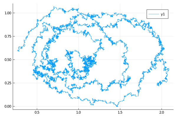
Note that we had to pass additional variables t, T and vT even though they are immaterial to the auxiliary law. The reason for this is that we defined LotkaVolterraAux in such a way that it is already fully compatible with GuidedProposals.jl and may be passed as an auxiliary law (and auxiliary laws currently require presence of fields t, T and vT). However, in practice, when dealing with LotkaVolterraAux, the internal states of t, T and vT are never used.