How to customize plots of diffusion trajectories?
Underneath a call to
X = ... # sampled trajectory
plot(X, Val(:x_vs_y))
# or
plot(X, Val(:vs_time))
Julia looks up the relevant plotting recipes implemented in DiffusionDefinition.jl in order to understand how the plot function should handle the object
X::TrajectoryHowever, in any other capacity, the called plot function behaves in an exactly the same way as if arrays with data were passed for plotting. In particular, you can pass additional named arguments as you would to a regular call to a plot function and change the plotting backend to anything supported by Julia.
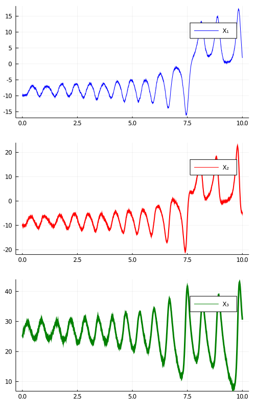
Example
For instance, using the law of the Lorenz–63 system we can decorate our plots as follows:
# change the backend if you want to
gr()

# plot
plot(
    X, Val(:vs_time);
    layout=(3, 1),
    size=(500, 800),
    label=["X₁" "X₂" "X₃"],
    color=["blue" "red" "green"],
    linewidth=[1 2 3]
)